Using internal functions of envfetch
using-internal-functions-of-envfetch.RmdOverview
There are multiple functions used by the main wrapper
envfetch function. If you’d like to use these, we have
replicated the main README.md functionality, using the internal
functions of envfetch, below.
1. Setup table of data with throw
Use of envfetch starts with a table: a dataframe,
tibble or sf object.
To begin, we need to create a data table containing a grid of points over Australia for a range of times.
For most applications, you will have your own dataset. If you have
your own data, load that in as a variable called d.
However, for this example, we can generate this using the
throw function.
The data set should look like this:
summary(d)## time_column geometry ## Intervals :100 POINT :100 ## Earliest endpoint:2017-01-01 epsg:4326 : 0 ## Latest endpoint :2017-01-02 +proj=long...: 0 ## Time zone :UTC
And can be visualized with a plot:
# load map of australia for reference
world <- ne_countries(scale = "medium", returnclass = "sf")
australia <- subset(world, admin == "Australia")

ggplot(data = australia) +
  geom_sf() +
  geom_sf(data = d, size = 1, show.legend = "point") +
  ggtitle("Australia with sample points") +
  theme_minimal()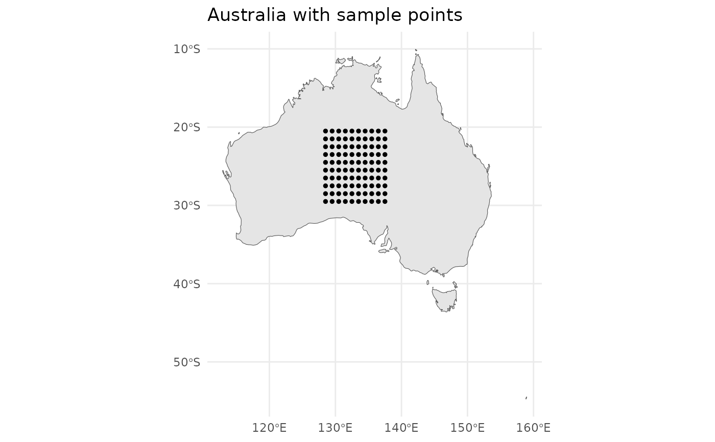
Each data point in the table has a sf::geometry object
along with a datetime (a lubridate::interval
or a date string). Ensure data used with the envfetch package matches
this format.
This geometry may be a point or a polygon. You may also
just use plain old x and y coordinates as
separate columns.
Each individual data point will use the datetime object
to decide what time range to extract and summarise data in.
datetime can be a time range
(lubridate::interval), a single date
(e.g. "20220101") or datetime
"2010-08-03 00:50:50".
2. Extract from your data sources with fetch
fetch:
- passes your data through your supplied extraction functions,
- caches progress, so that if your function crashes somewhere, you can continue where you left off and
- allows you to repeat sampling across different times (see section 3, below).
You can supply any data extraction function to fetch,
but some useful built-in data extraction functions are provided:
| Function name | Description |
|---|---|
extract_over_time |
Extract and summarise raster data over multiple time periods for each row in your dataset. |
extract_over_space |
Extract and summarise raster data over space for each row in your dataset. |
extract_gee |
Use Google Earth Engine to extract your chosen image collection bands and summarise this information for each row in your dataset. |
get_daynight_times |
Calculates the time since sunrise, time since sunset and day and night hours for each row in your dataset. |
Note, the get_daynight_times function provides an
example of how you could extend the caching mechanism of
envfetch for a purpose other than extracting data from
raster files.
In this example, we will use:
extract_over_timeto extract from a large pre-downloaded NetCDF fileextract_geeto extract NDVI data from the MODIS MOD13Q1 dataset on Google Earth Engine
To fetch the data, use the fetch
function and supply it with the extraction functions you would like to
use. You can supply your own custom function here, but ensure you use
the anonymous function syntax so you can specify custom arguments. That
is, if following purrr formula syntax:
~your_function(.x, custom_arg='arg_value') or if following
base R,
function(x) your_function(x, custom_arg='arg_value')).
Note, .x in the below example is your data set,
d.
extracted <- d |>
  fetch(
    ~extract_over_time(.x, r = '/path/to/netcdf.nc'),
    ~extract_gee(
       .x,
       collection_name='MODIS/061/MOD13Q1',
       bands=c('NDVI', 'DetailedQA'),
       time_buffer=16,
     )
  )
3. Obtain data for repeated time intervals
In certain applications, you may need to obtain environmental data
from repeated previous time periods. For example, we can extract data
from the past six months relative to the time (start time if an interval
is provided) of each data point, with an average calculated for each
two-week block, using the .time_rep
variable.
rep_extracted <- d |>
  fetch(
    ~extract_over_time(.x, r = '/path/to/netcdf.nc'),
    ~extract_gee(
       .x,
       collection_name='MODIS/061/MOD13Q1',
       bands=c('NDVI', 'DetailedQA'),
       time_buffer=16,
     ),
    .time_rep=time_rep(interval=lubridate::days(14), n_start=-12),
  )
Integrate other packages and create your own fetch function
In some cases, you may want to combine envfetch with other third party tools. Below, we will illustrate how to do this with the weatherOz R package. Visit the link to see their project details and licensing.
# install.packages("weatherOz", repos = "https://ropensci.r-universe.dev")
library(weatherOz)
library(envfetch)
library(tidyverse)
library(cli)

# authenticate with SILO using the weatherOz package
get_key(service = "SILO")

# make a wrapper function to adapt weatherOz for envfetch data inputs
get_data_drill_wrapper <- function(x, summary_fn=mean) {
  points <- sf::st_centroid(x)
  coords <- sf::st_coordinates(points) %>%
    as_tibble()

  cli_progress_step("Fetching weather data for {nrow(coords)} location{?s}")

  results <- map(1:nrow(coords), function(i) {
    cli_progress_message("Processing location {i}/{nrow(coords)}")

    start_date <- as.Date(lubridate::int_start(x$time_column[i]))
    end_date <- as.Date(lubridate::int_end(x$time_column[i]))

    # use a tryCatch as requests with no result raise errors
    # we just want NAs in those cases.
    result <- tryCatch({
      dat <- get_data_drill(
        latitude = coords$Y[i],
        longitude = coords$X[i],
        start_date = start_date,
        end_date = end_date
      )
      # aggregate the data for this location
      summarised <- dat %>%
        select(-any_of(c("date", "latitude", "longitude", "date", "extracted"))) %>%
        summarise(
          # summarise everything except elevation
          across(-elev_m, ~ summary_fn(.x, na.rm = TRUE)),
          # special-case elevation: strip " m", convert numeric, summarise
          elev_m = summary_fn(as.numeric(gsub(" m$", "", elev_m)), na.rm = TRUE)
        )
      return(summarised)
    }, error = function(e) {
      cli_alert_warning("Error for location {i}: {e$message}")
      # return a row with NAs but proper structure
      return(tibble(
        latitude = coords$Y[i],
        longitude = coords$X[i],
        date = as.Date(NA),
        max_temp = NA_real_,
        min_temp = NA_real_,
        rain = NA_real_
      ))
    })

    return(result)
  })

  combined_results <- bind_rows(results)
  combined_results <- combined_results
  return(combined_results)
}


# extract with the `fetch` function from `envfetch`
extracted_weatherOz <- d[1:5,] %>%
  fetch(
    ~get_data_drill_wrapper(.x, mean),
    use_cache = FALSE
  )
Then, if you want to obtain that environmental data from repeated previous time periods, you can again add the time_rep value.
Here we extract data from the past six months relative to the time
(start time if an interval is provided) of each data point, with an
average calculated for each two-week block, using the
.time_rep variable.
# extract with the `fetch` function from `envfetch`
# and repeat extractions calculating averages for each two-week block for the last
# 6 months
extracted_weatherOz <- d[1:5,] %>%
  fetch(
    ~get_data_drill_wrapper(.x, mean),
    use_cache = FALSE,
    .time_rep=time_rep(interval=lubridate::days(14), n_start=-12)
  )